Exploring Reinforcement Learning in Agent-Based Modeling
Table of contents
- Topic and Problem Description
- Real-Life Comparison
- Purpose of the Study
- Algorithm Description
- Conclusion
- Appendix
Topic and Problem Description
Understanding the allocation of resources such as schools, hospitals, and public services is crucial in addressing socio-economic issues. In urban planning, it’s vital to ensure that people have adequate access to these essential resources. The challenge lies in creating a model that can simulate how agents—representing individuals or families—navigate their environment and make decisions based on their proximity to these resources. This is where reinforcement learning (RL) can play a transformative role.
Real-Life Comparison
Imagine a city where families are trying to choose housing locations based on the proximity to schools, hospitals, and parks. Families with children may prioritize living near good schools, while elderly individuals might look for access to healthcare facilities. By simulating this behavior, we can better understand the dynamics of resource allocation and how different socio-economic factors influence where people choose to live.
Purpose of the Study
The objective of this project is to develop a reinforcement learning framework that allows agents to intelligently adapt their strategies when searching for housing near important resources. By simulating these behaviors, we aim to gain insights into optimal resource placement and how to reduce disparities in access to essential services. This research contributes to more effective urban planning and resource allocation strategies.
Algorithm Description
Our approach employs a Q-learning algorithm within an agent class, structured as follows:
-
State Representation: Each agent \( i \) at time \( t \) is represented by its position in a continuous grid: \(\mathbf{s}_i(t) = (x_i(t), y_i(t))\)
-
Q-Table Initialization: Each agent maintains a Q-table that encodes its knowledge of state-action values: \(Q: \mathbb{R}^{(G \times 10) \times (G \times 10) \times 4}\) where \( 4 \) corresponds to the available actions: left, right, up, and down.
-
Action Selection: Agents select actions based on an exploration-exploitation strategy: \(a_i(t) = \begin{cases} \text{random} & \text{with probability } \epsilon(t) \\ \arg\max_a Q(\mathbf{s}_i(t), a) & \text{otherwise} \end{cases}\)
-
Movement Mechanics: Agents are encouraged to move towards the nearest resource while also avoiding edges of the grid.
- Reward Calculation: The reward function includes:
- Exploration Bonus: Encouraging agents to explore their environment.
- Proximity Reward: Higher rewards for being closer to essential resources. \(r_i(t) = r_{exploration} + \sum_{j=1}^{M} R_{proximity}(d_{ij}) + R_{zone}(d_{ij})\)
- Q-value Update: The Q-value for each action is updated based on the rewards received: \(Q(\mathbf{s}_i(t), a_i(t)) \leftarrow Q(\mathbf{s}_i(t), a_i(t)) + \alpha \left( r_i(t) + \gamma \max_a Q(\mathbf{s}_i(t + 1), a) - Q(\mathbf{s}_i(t), a_i(t)) \right)\)
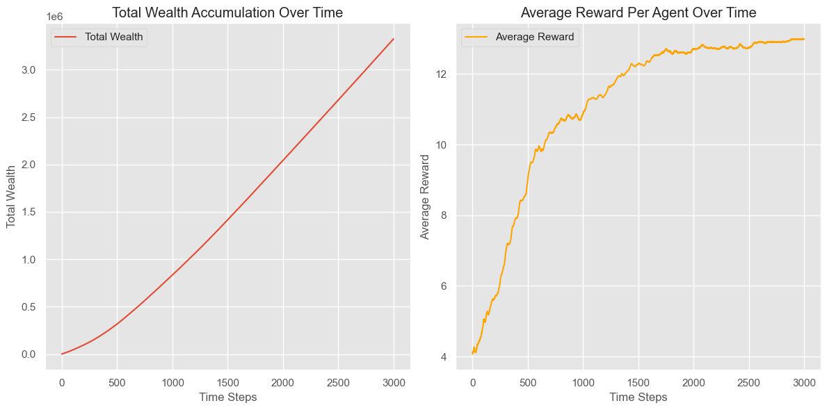
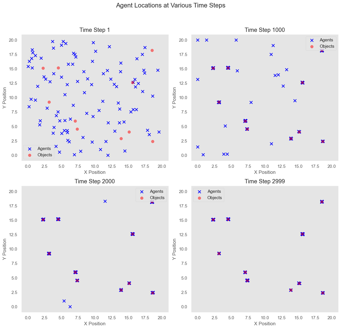
The following plots show the accumulated total wealth of the agents, the average rewards per iteration, and the paths of the agents at different time steps compared to the locations of the objects.
Conclusion
This project utilizes reinforcement learning to empower agents in navigating a simulated urban environment. By understanding how agents allocate their locations based on access to essential resources, we can devise better strategies for urban planning and resource distribution. This study not only enhances the field of agent-based modeling but also informs future decisions in socio-economic policy-making and resource allocation. Through this approach, we aim to create a more equitable distribution of essential services and improve overall quality of life for urban residents.
Appendix
import tqdm
import numpy as np
import random
import matplotlib.pyplot as plt
# Environment parameters
NUM_AGENTS = 100
NUM_OBJECTS = 10
TIME_STEPS = 3000
GRID_SIZE = 20.0 # Continuous grid size
NUM_ACTIONS = 4 # Actions: left, right, up, down
# Global variable to store objects
global_objects = None
# Initialize global variables for tracking performance metrics
total_wealth_per_time_step = np.zeros(TIME_STEPS)
average_rewards_per_time_step = np.zeros(TIME_STEPS)
agent_positions_history = [] # Track agent positions over time
# Agent class
class Agent:
def __init__(self, x, y):
self.x = x
self.y = y
self.q_table = np.zeros((int(GRID_SIZE * 10) + 1, int(GRID_SIZE * 10) + 1, NUM_ACTIONS))
self.learning_rate = 0.1
self.discount_factor = 0.95
self.exploration_rate = 1.0
self.exploration_decay = 0.99 # Slower decay to encourage exploration
self.total_wealth = 0
def choose_action(self):
if random.uniform(0, 1) < self.exploration_rate:
return random.randint(0, NUM_ACTIONS - 1) # Explore
return np.argmax(self.q_table[int(self.x * 10), int(self.y * 10)]) # Exploit
def update_exploration_rate(self):
self.exploration_rate = max(0.1, self.exploration_rate * self.exploration_decay)
def update_q_value(self, action, reward, next_state):
best_future_q = np.max(self.q_table[int(next_state[0] * 10), int(next_state[1] * 10)])
current_q = self.q_table[int(self.x * 10), int(self.y * 10), action]
self.q_table[int(self.x * 10), int(self.y * 10), action] += self.learning_rate * (
reward + self.discount_factor * best_future_q - current_q)
def update_wealth(self, reward):
self.total_wealth += reward
return self.total_wealth
def move(self, action):
step_size = 0.1 # Continuous movement step size
near_objects = [obj for obj in global_objects if np.sqrt((self.x - obj[0])**2 + (self.y - obj[1])**2) < 1]
# If near an object, consider moving towards it
if near_objects:
# Move towards the closest object
closest_obj = min(near_objects, key=lambda obj: np.sqrt((self.x - obj[0])**2 + (self.y - obj[1])**2))
direction_x = closest_obj[0] - self.x
direction_y = closest_obj[1] - self.y
direction_length = np.sqrt(direction_x**2 + direction_y**2)
if direction_length > 0:
self.x += (direction_x / direction_length) * step_size
self.y += (direction_y / direction_length) * step_size
return # Exit after moving towards an object
# Regular movement if not near any objects
if action == 0: # left
self.x = max(0, self.x - step_size)
elif action == 1: # right
self.x = min(GRID_SIZE, self.x + step_size)
elif action == 2: # down
self.y = max(0, self.y - step_size)
elif action == 3: # up
self.y = min(GRID_SIZE, self.y + step_size)
# Add a penalty for moving towards the edges
if self.x <= 0 or self.x >= GRID_SIZE or self.y <= 0 or self.y >= GRID_SIZE:
self.update_wealth(-0.1) # Small penalty for edge movement
# Function to create objects
def create_objects(num_objects):
return [(random.uniform(0, GRID_SIZE), random.uniform(0, GRID_SIZE)) for _ in range(num_objects)]
# Function to calculate rewards with improved structure
def calculate_reward(agent, objects):
reward = 0
exploration_bonus = 0.01 # Small reward for exploration
close_enough_reward_base = 5.0 # Base reward when within 5 units
reward_zone_radius = 3.0 # Define the radius of the reward zone
# Add exploration bonus
reward += exploration_bonus
for obj in objects:
distance = np.sqrt((agent.x - obj[0])**2 + (agent.y - obj[1])**2)
if distance <= 5: # Within 5 units
# Calculate reward based on proximity
proximity_reward = close_enough_reward_base * (1 - (distance / 5)) # Increases as they get closer
reward += max(proximity_reward, 0) # Ensure non-negative reward
# Reward zone bonus
if distance <= reward_zone_radius: # Check if within reward zone
additional_reward = (reward_zone_radius - distance) * (close_enough_reward_base / reward_zone_radius)
reward += max(additional_reward, 0) # Ensure non-negative reward
return reward
# Update the run_simulation function to track performance metrics
def run_simulation():
global global_objects # Declare the global variable
agents = [Agent(random.uniform(0, GRID_SIZE), random.uniform(0, GRID_SIZE)) for _ in range(NUM_AGENTS)]
global_objects = create_objects(NUM_OBJECTS) # Create objects and store them globally
for t in tqdm.tqdm(range(TIME_STEPS)):
total_rewards = 0
positions = [(agent.x, agent.y) for agent in agents] # Capture agent positions
for agent_index, agent in enumerate(agents):
current_state = (agent.x, agent.y)
action = agent.choose_action()
agent.move(action)
next_state = (agent.x, agent.y)
reward = calculate_reward(agent, global_objects)
# Update wealth and total rewards
agent.update_wealth(reward)
total_rewards += reward
agent.update_q_value(action, reward, next_state)
# Update exploration rate
agent.update_exploration_rate() # Update exploration rate here
# Track performance metrics
total_wealth_per_time_step[t] = sum(agent.total_wealth for agent in agents)
average_rewards_per_time_step[t] = total_rewards / NUM_AGENTS
agent_positions_history.append(positions) # Store positions history
# ===================== Plotting ===================== #
def plot_results():
plt.figure(figsize=(12, 6))
# Plot total wealth accumulation
plt.subplot(1, 2, 1)
plt.plot(total_wealth_per_time_step, label='Total Wealth')
plt.title('Total Wealth Accumulation Over Time')
plt.xlabel('Time Steps')
plt.ylabel('Total Wealth')
plt.legend()
# Plot average rewards
plt.subplot(1, 2, 2)
plt.plot(average_rewards_per_time_step, label='Average Reward', color='orange')
plt.title('Average Reward Per Agent Over Time')
plt.xlabel('Time Steps')
plt.ylabel('Average Reward')
plt.legend()
plt.tight_layout()
plt.show()
def plot_agent_locations(time_steps):
fig, axs = plt.subplots(2, 2, figsize=(12, 12))
fig.suptitle('Agent Locations at Various Time Steps', fontsize=16)
for idx, time_step in enumerate(time_steps):
agents_positions = np.array(agent_positions_history)[time_step]
axs[idx // 2, idx % 2].scatter(agents_positions[:, 0], agents_positions[:, 1], color='blue', label='Agents', marker='x', s=50) # Change to X marker
axs[idx // 2, idx % 2].scatter(*zip(*global_objects), color='red', alpha=0.5, label='Objects', s=50)
axs[idx // 2, idx % 2].set_xlim(-1, GRID_SIZE + 1)
axs[idx // 2, idx % 2].set_ylim(-1, GRID_SIZE + 1)
axs[idx // 2, idx % 2].set_title(f'Time Step {time_step}')
axs[idx // 2, idx % 2].set_xlabel('X Position')
axs[idx // 2, idx % 2].set_ylabel('Y Position')
axs[idx // 2, idx % 2].legend()
axs[idx // 2, idx % 2].grid()
plt.tight_layout(rect=[0, 0.03, 1, 0.95])
plt.show()
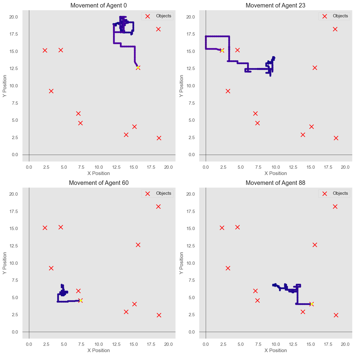
def plot_multiple_agents_movements(agent_indices):
num_agents = len(agent_indices)
num_steps = len(agent_positions_history)
plt.figure(figsize=(12, 12))
object_positions = np.array(global_objects)
for idx, agent_index in enumerate(agent_indices):
agent_movements = np.array(agent_positions_history)[:, agent_index] # Get positions for the specific agent
# Create a color gradient from white to black
colors = plt.cm.plasma(np.linspace(0, 1, num_steps))
# Create subplot for each agent
plt.subplot(2, 2, idx + 1)
# Plot the agent's movement
for i in range(num_steps - 1):
plt.plot(agent_movements[i:i + 2, 0], agent_movements[i:i + 2, 1], color=colors[i], marker='o', markersize=3)
# Plot the objects
plt.scatter(object_positions[:, 0], object_positions[:, 1], color='red', label='Objects', marker='x', s=100)
plt.title(f'Movement of Agent {agent_index}')
plt.xlim(-1, GRID_SIZE + 1)
plt.ylim(-1, GRID_SIZE + 1)
plt.xlabel('X Position')
plt.ylabel('Y Position')
plt.axhline(0, color='black', lw=0.5)
plt.axvline(0, color='black', lw=0.5)
plt.grid()
plt.legend()
plt.tight_layout() # Adjusts subplot parameters to give specified padding
plt.show()